ANOVA for Visual Learners
Almost everything in this world has some variability. A bit of randomness that makes one flower different, one dog look different, and each person unique. In statistics, we leverage this randomness when creating models and testing hypotheses. This blog post is the first of a series visually working through different statistical models. I am going to start with ANOVA as it is one of the most basic models and often times the first model people are introduced to.
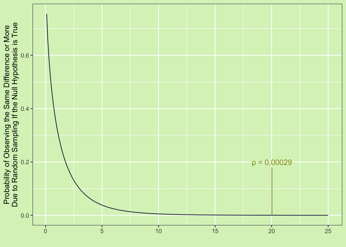
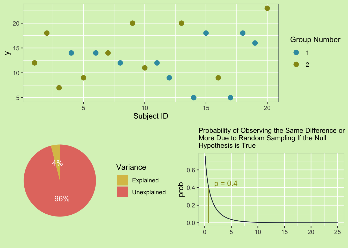
The basic question of the ANOVA model is: “Does the mean of group one equal to the mean of group two?”. You might be wondering why testing the means of two groups has anything to do with variance. And hey, that is a fair question. The reason they are connected is because of the law of total variance, which basically says variance comes in two kinds; the explained and the unexplained. If we can figure out how much of the variance of the thing we are measuring is due to the groups (i.e. explained) and how much of the variance is just random chance (i.e. unexplained) then we can get the probability the two groups are the same. If that probability is low then we can reject the notion that the two groups are the same.
Example Data
Now as promised some plots. First let’s start with the scenario where the groups are truly different and have a low variance.
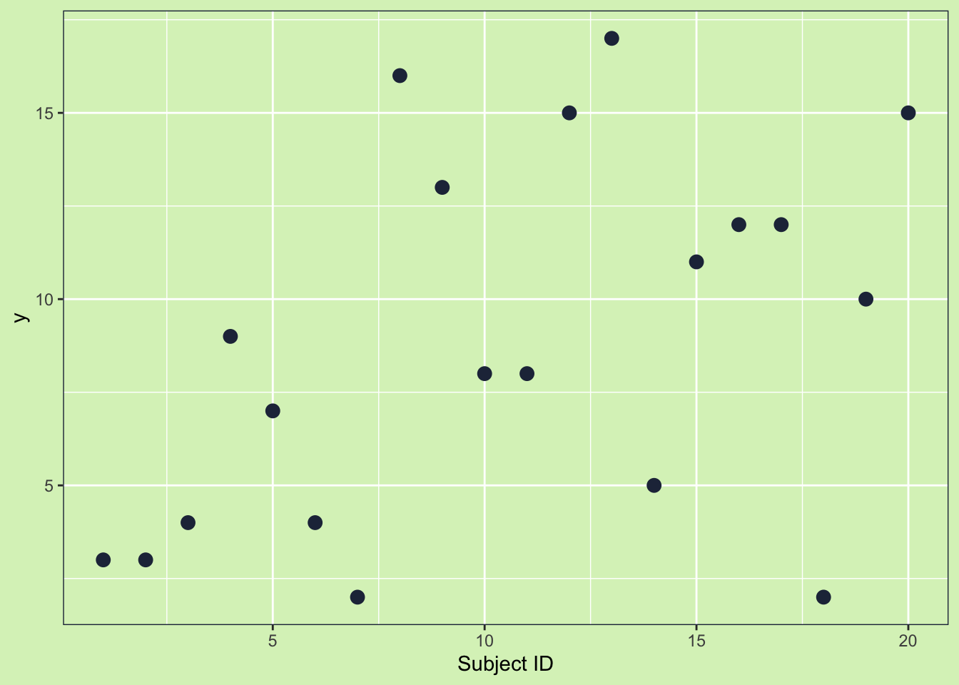 Looking at the plot there are 20 data points with a variability of 24.5. It isn’t super clear that two groups make up the data, but let’s add some color to tell the two groups apart.
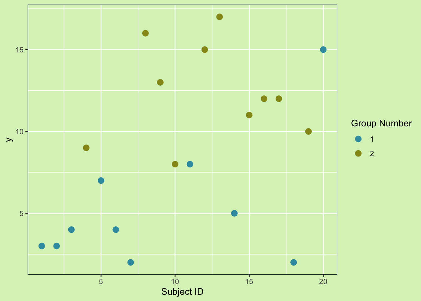
Now we can clearly see group 2 has higher values than group 1. This means that at least some of the variability we see in y can be explained by the groups! This happens all the time in real life. For example if I were to weigh some apples and pineapples, then part of variability in the weights would be due to the fact that pineapples and apples are different fruits. So we can explain that part of the variability. The same is happening here. We measured y, which had a variability of 24.5. From looking at the plot we can see it is like the groups are causing some of the variability, but now the question is how much. To answer that question we are going to need to do an Analysis Of VariAnce (ANOVA)
The basic equation we use in ANOVA is:
\[ SS_{Total} = SS_{Explained}+SS_{Unexplained}\]
Where \(SS_*\) stands for sum of squares. The sum of squares is a unscaled measure of variability.
Total Sum of Squares
Graphically, variability is just the distance between two points. So if we want to look at the total sum of squares, the first step is to get a sense of the how each point varies from the overall mean. We do this by getting the distance between each point and the mean. This distance is called the residual. Each residual is represented below on the plot, with an orange dashed line.
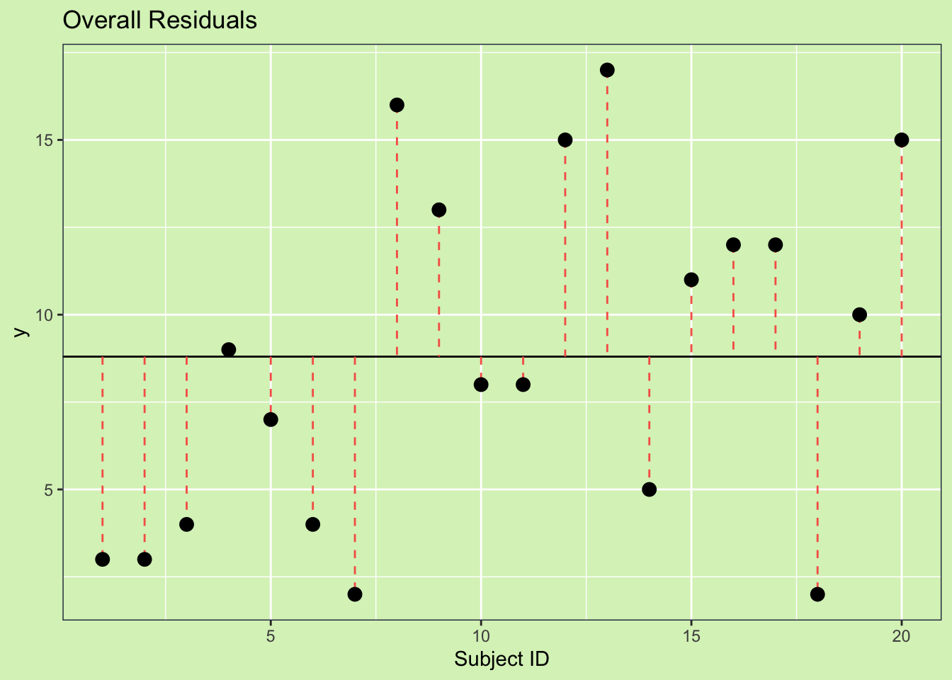 To get a single number we are going to add up all the residuals, but because the residuals are always the value minus the mean (\(r = y - \hat{y}\)), we have to square this value so it is always positive. Adding together all of these squared residuals gives us the total deviation from the mean.
This value is the sum of square \(SS_{Total}\). The equation for this is:
\[SS_{Total} = \sum{(X_{ij}-\bar{X})}\]
Unexpalined Sum of Squares
To calculate the unexplained variability we need to figure out how much deviation is left over when we do account for groups. We do this by measuring For the variance not explained by the groups. The calculation is basically the same as the \(SS_{Total}\), but instead of using the overall mean we use the group means. We can see this graphically by drawing the within group residuals.
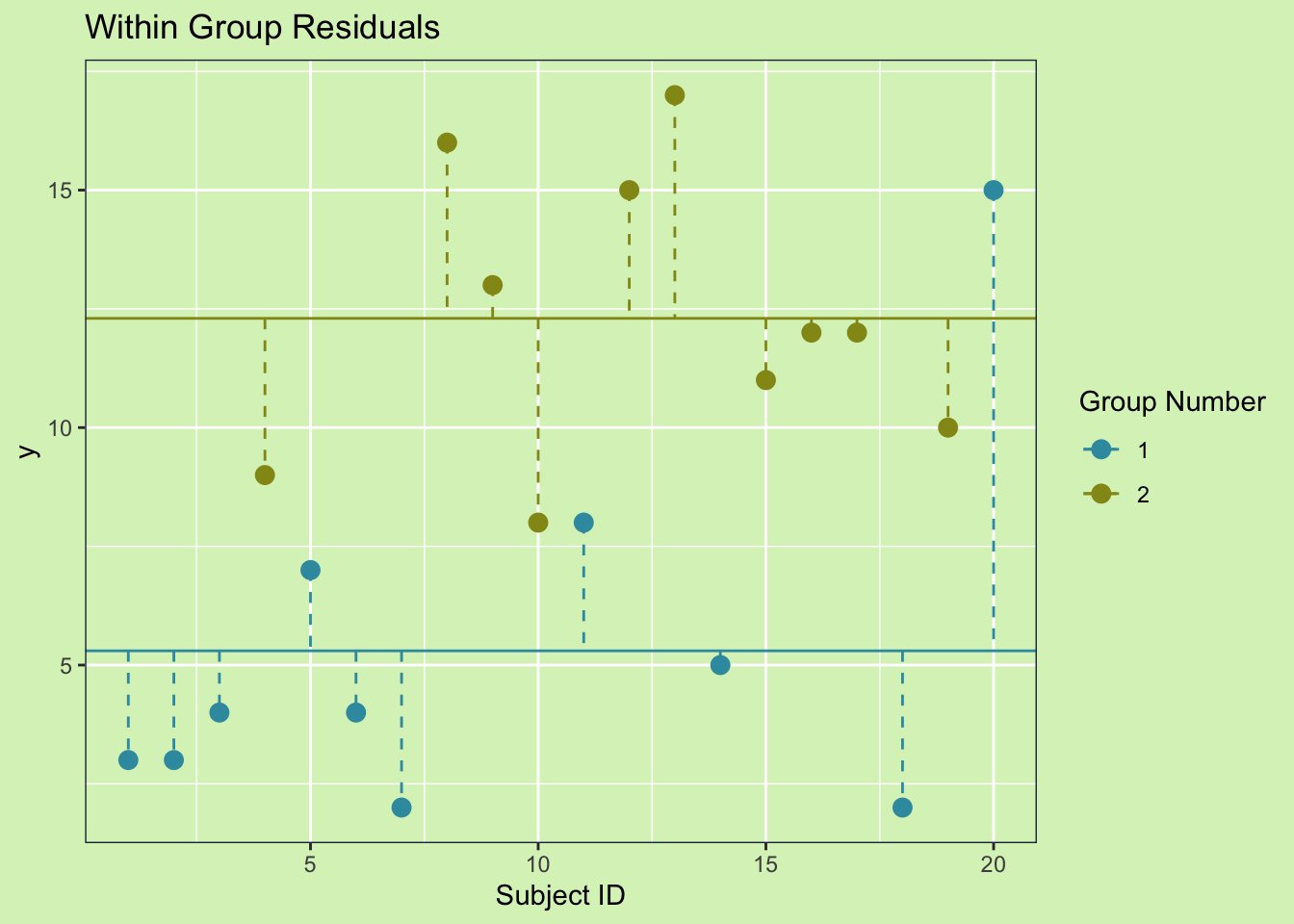
This shows the unexplained variance because the difference between one groups mean and the overall mean is the explained variance. So, after accounting for the different means of each group, any left over variability is considered unexplained. As before, to get the sum of squares, we square each residual and sum them. The equation is as follows:
\[SS_{Unexplained} = \sum{(X_{ij}-\bar{X_j})}\]The value is also called the sum of squares within groups, or sum of squares of the error.
\[SS_{Unexplained} = SS_{Within} = SS_{Error}\]
### Sum of Squares Explained
Graphically the explained variance is the distance between the mean of the groups and the overall mean. We can create this by combining the two plots above and drawing our residual lines between the mean of the groups and the mean overall.
 Just like the previous sum of squares equations, we need to square the residuals and add them up. The one difference is because we are using means. Means contain information from multiple points, so we need to account for that by multiplying by the number of subjects in each group. This makes the equation as follows:
Now we have all the parts we can put them togther graphically and see how it works. The original equation is: \[ SS_{Total} = SS_{Explained}+SS_{Unexplained}\] The sum of squares explained is also known as sum of squares between groups and sum of squares treatment. \[SS_{Explained} = SS_{Between} = SS_{Treatment}\]
Sum of Squares Equation
If we follow a single subject we can see how this all adds together.
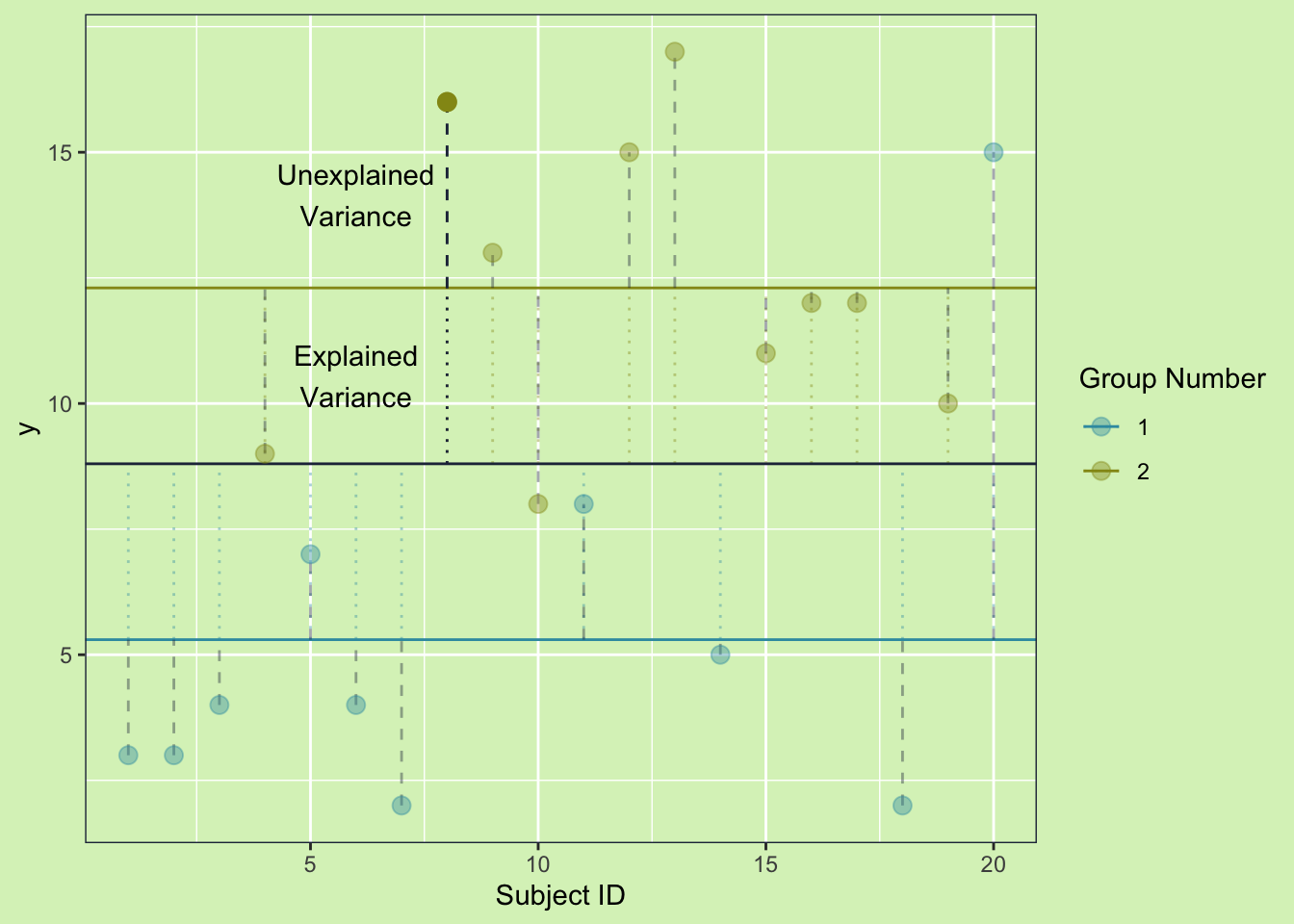 From the first plot we saw that the \(SS_{Total}\) is calculated by measuring the distance from the overall to a point. And we can see how the \(SS_{Expained}\) and the \(SS_{Unexpained}\) add together to equal the \(SS_{Total}\)
With the basic sum of squares equation defined we can start to answer our original question.
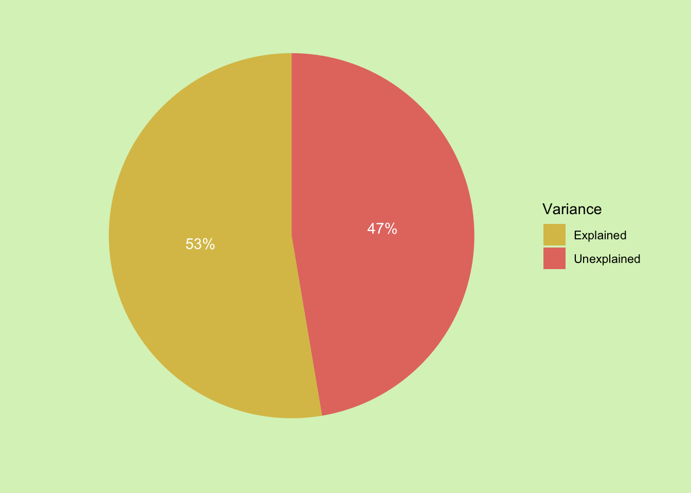
The first question of what proportion of the variance can be explained is solved by just taking the explained sum of squares as a proportion of the total sum of squares. This is usually called eta \[\eta = \frac {SS_{Explained}} {SS_{Total}}\] So for this sample the groupings explain 53% of the observed variance. We can make a quick pie chat to show this:
